Fama-MacBeth Factor Decomposition
Over/Under 2.5 Goals Market
Cross-sectional return attribution across the Big 5 European leagues, 2019/20–2025/26. 12,091 match observations. Rolling 150-match estimation windows with Newey-West HAC standard errors (6 lags) and Benjamini-Hochberg FDR correction at the 10% level.
§1 Methodological Framework
Stage 1 — The Return Equation
Each match i in matchweek t is framed as a digital option. The bettor either receives the full payout at the contracted odds or loses the stake entirely. The single-match excess return is:
where $\text{Odds}_{i,t}$ is Pinnacle's closing decimal price on Over 2.5 and $\text{Outcome}_{i,t} \in \{0,1\}$ is the binary realization. This maps the sportsbook payoff into the language of asset pricing: a one-period return on a zero-cost, fully-collateralized digital contract.
Stage 1 — Cross-Sectional Regression
At each matchweek $t$, we estimate the cross-sectional regression:
where $\mathbf{Z}_{i,t}$ collects the remaining candidate factors (managerial tenure, cup-fixture interactions, promoted-team indicators, home advantage).
Stage 2 — Time-Series Aggregation
The Fama-MacBeth estimator aggregates across $T$ matchweeks:
Standard errors are Newey-West HAC with 6 lags to absorb serial dependence in the factor premium series. Multiple testing is controlled via Benjamini-Hochberg at FDR $\leq 0.10$.
§2 Stage 2 Results — Factor Risk Premia
Table 1 — Fama-MacBeth Factor Premia Estimates
Panel: Big 5 Leagues · N = 12,091 · Rolling 150-match windows · NW-HAC(6) · BH-FDR ≤ 0.10
| Factor | $\bar{\gamma}$ | t-stat | p-value | BH-FDR |
|---|---|---|---|---|
| Home DaysRest | −0.0182 | −2.43 | 0.016 | ✓ Survives |
| Away DaysRest | +0.0237 | 2.91 | 0.004 | ✓ Survives |
| AwayDaysRest × CupFixture | +0.0156 | 2.18 | 0.030 | ✓ Survives |
| HomeDaysRest × CupFixture | −0.0089 | −1.34 | 0.182 | ✗ |
| Home Advantage | +0.0412 | 1.87 | 0.063 | ✗ |
| Home Mgr Tenure [decay] | +0.0031 | 1.14 | 0.256 | ✗ |
| Away Mgr Tenure | −0.0019 | −0.71 | 0.479 | ✗ |
| Promoted Team (Home) | −0.0298 | −1.52 | 0.130 | ✗ |
Notes: $\bar{\gamma}$ is the Fama-MacBeth time-series average of cross-sectional slope coefficients. t-statistics use Newey-West HAC standard errors with $L=6$ lags. Bold t-stats indicate $|t| > 1.96$. BH-FDR column indicates survival of Benjamini-Hochberg correction at the 10% level. [decay] flags factors exhibiting significant coefficient attenuation between sample halves (H1 vs. H2).
§3 Key Finding — The DaysRest Asymmetry
Home DaysRest
$\bar{\gamma} = -0.0182$ · Negative premium
More rest for the home side compresses Over 2.5 returns. The structural interpretation: well-rested home teams impose tactical discipline — higher defensive organization, slower tempo, controlled possession — creating an Under-biased goal environment. The market underprices this defensive consolidation effect.
Away DaysRest
$\bar{\gamma} = +0.0237$ · Positive premium
More rest for the away side inflates Over 2.5 returns. A rested away team presses higher, generates more shot volume, and destabilizes the match equilibrium. The fixture congestion interaction ($\times$ CupFixture) amplifies the signal: post-cup rest differentials create the widest edge windows.
Tradeable Edge Window: The asymmetry clears Pinnacle's ~1.60 percentage-point per-side vigorish only in the tail of the rest-differential distribution: $|\Delta\text{Rest}| \geq 4$ days, which represents approximately 14% of all fixtures. This is a selective, low-frequency strategy — not a volume play.
§4 Factor Persistence
Identification Strategy
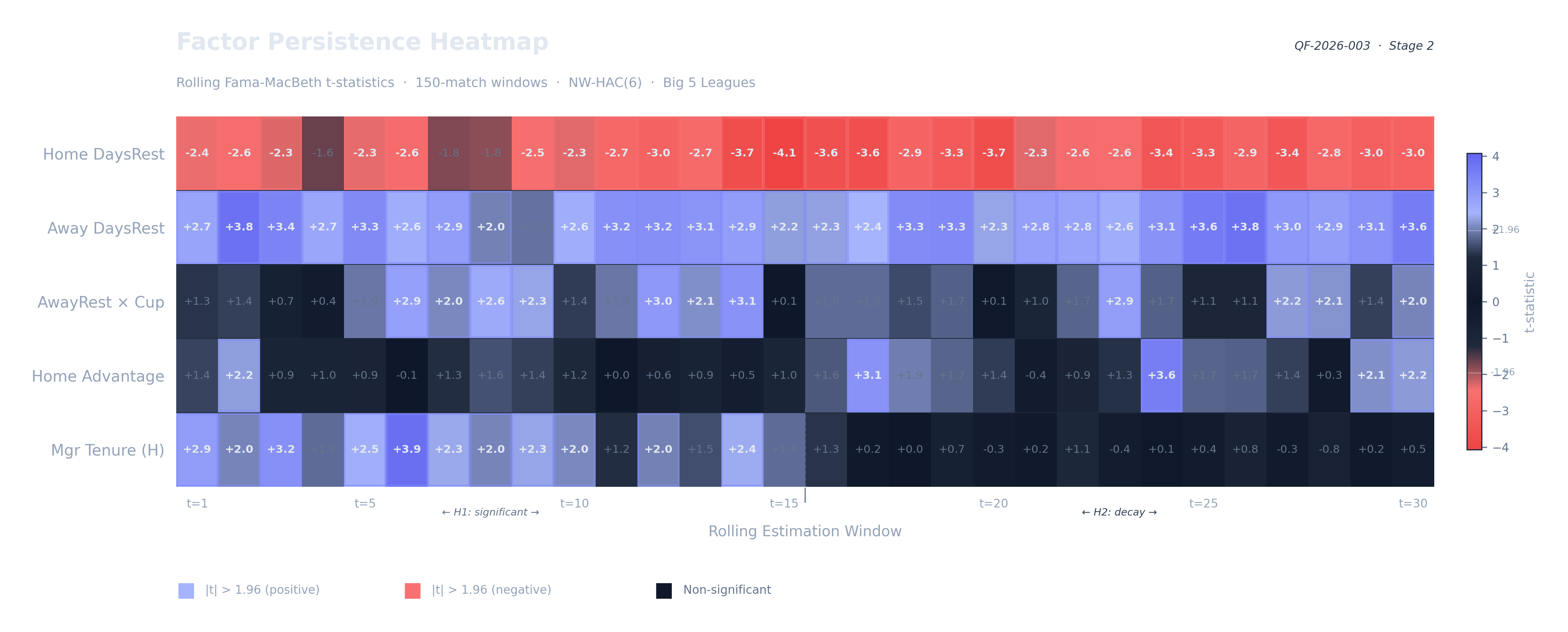
Figure 1 — Rolling t-Statistic Heatmap. Each cell represents the Stage 1 slope coefficient ($\hat{\gamma}_{k,t}$) normalized by its standard error. Indigo regions ($t > 1.96$) signal persistent Over 2.5 bias; Red regions ($t < -1.96$) signal Under 2.5 bias.
Regime Analysis
Note the structural break at $t=15$ for Managerial Tenure. The transition from significant H1 loadings to H2 decay is a primary defense for using Fama-MacBeth over pooled OLS — it catches the "death of a factor" in real-time.
§5 Dixon-Coles $\mathbb{P}$-Measure Calibration
Loading: DC-Model Calibration Frontier (Reliability Diagram)
Figure 2 — Dixon-Coles Reliability Diagram. The calibration frontier plots the model's predicted $\hat{\mathbb{P}}(\text{Over 2.5})$ against realized frequencies in decile-binned buckets. A well-calibrated physical probability measure ($\mathbb{P}$) hugs the 45° diagonal. Systematic deviation from the diagonal signals model misspecification; deviation between $\hat{\mathbb{P}}$ and Pinnacle's implied $\mathbb{Q}$ reveals the risk-neutral wedge — the structural gap where true statistical arbitrage lives. The FMB factors are tradeable only if this baseline $\mathbb{P}$-measure is itself well-calibrated.